Lec #24: SDPs I

• Nicholas asked how, in the SoS example where we wanted to write
  the polynomial

  

  as a sum of square polynomials, we could quickly restrict ourselves to
  .

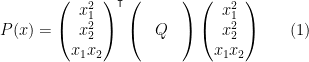
  Here’s one way. Of course, in general we have to consider the vector , since the squares of these monomials span . This means we must consider a much larger (i.e., ) matrix , and try to write with . But observe two simple facts:

  • The first three diagonal terms of are zero, by inspection.
  • The bottom principal minor is just our old matrix.

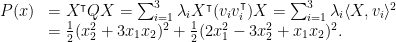
  Now we claim that if some diagonal term in some PSD matrix is zero, then all entries in that row and column are zero too. Indeed, if , then for any , the non-negativity of the determinants of the principal minors (see below) says: , so . Hence, the problem just collapses to finding such that

  

  which we saw a solution for. Indeed, if we set

  

  then the eigenvalues are , with eigenvectors

  

  Since , you get

  

  Which is the SoS representation we wanted.

• Thanks, C.J.: I’d clean forgotten about the all-important equivalent definition of PSD-ness: is PSD if and only if all principal minors have non-negative determinants. Recall that a principal minor is obtained by restricting to some set of rows and columns. One direction of the proof is easy (and thankfully it’s the one we need): first, a matrix is PSD then all its principal minors are PSD. (Use the definition.) But the determinant of a principal minor is just the product of its eigenvalues, which is non-negative for PSD matrices. The other direction is a little more involved, I don’t know a one-line proof, please consult your favorite algebra text. (Or if you know one, catch me and tell me about it.)

• Finally, the point that Goran asked a clarification for: if has max-degree , then the need only be polynomials of degree at most . Suppose not. Let be the highest degree monomial in some , and let contain all the monomials in of degree . Now is a sum of square polynomials, and all its terms (of degree ) also appear in .

  Goran had asked: Can be identically zero, with all its terms cancelling out? No, and here’s one easy way to see it: consider some for which some . Then . (I am sure there are another easy arguments? Please tell me about them.)

Lec #19: JL etc.

So two things that we wanted to check during lecture today, and some notes:

• If is sub-Gaussian with parameter , and they are independent, then is indeed sub-Gaussian with parameter , as claimed. Basically, just use the MGF definition to show this. And note the analogy to Gaussians, where should be the standard deviation, and not the variance.
• I got the sub-exponential equivalence slightly wrong. The MGF-based definition: there exist parameters such that

  

  This is equivalent to there existing some other constants such that

  

  See Theorem~2.2 here for a proof. (Thanks for pointing out that mistake, Tom!)

• For compressive sensing, there are a million resources online. E.g., here’s Terry Tao on the topic.
• I should have emphasized: the blood testing example we talked about was the simple case where you were guaranteed that the vector was -sparse. I.e., there is exactly one person with the disease among a population of people. Then the binary search strategy we did used linear tests, which is optimal. (To clarify, for each , the test combines together the samples for all people whose index has a in the place and tests this combination. Now construct a -bit vector with a in the position precisely if the test came up positive: this is the index of the person with the infection.

  Note this is a non-adaptive strategy: we can write down all the tests up-front, and can read off the answer from their results. This is opposed to an adaptive strategy that would look at the answers to previous tests to decide which sets to test next.

  What about the case where there are exactly two people infected? The same strategy does not work. In fact, since there are answers and each answer gives us bit each time, we must perform at least tests. Any thoughts on how to do this? An adaptive strategy that uses tests is easy: can you get a non-adaptive strategy? Using randomness?

Matroids

Some of you asked for intuition about matroids: they seem so abstract, how to think about them? Whenever I have to prove a fact about matroids, I think about how I’d prove the fact for graphic matroids. And often (though alas, not always) that proof translates seamlessly to general matroids.

Recall that a graphic matroid is constructed as follows: take a graph. Its edges are the elements of the matroid. A set of elements (edges) is independent if they do not induce a cycle (in the graph-theory sense), i.e., if they form a forest. Now you can check that this definition satisfies the conditions for being a matroid. The bases of the matroid are spanning trees of G.

So on HW3, the first part asked: suppose I have two spanning trees on a graph G, a red one and a blue one. Show that there exists a bijection F between the red and blue edges so that replacing any red edge e by its matched blue edge F(e) gives a spanning tree. The proof now seems well within reach. And the arguments to prove it (adding an element/edge forms a cycle, etc) all generalize to matroids.

Why are we studying matroids? They form a convenient abstraction for many combinatorial structures you often encounter. E.g., spanning trees, linearly-independent sets of vectors, matchable vertices in a bipartite graph, sets of vertices that can routed to a sink in some vertex-disjoint way, all are matroids. E.g., perfect matchings in bipartite graphs can be phrased as finding a common base of two matroids defined on the same ground set. A famous result of Edmonds shows that this matroid intersection problem can be solved for any two matroids. Also, since matroids characterize the greedy algorithm (in a sense you saw in HW1), the fact that the greedy algorithm works for some problem often indicates there may be some deeper structure lurking within, that we can exploit.

I was hoping to cover matroids in a lecture later in the course (let’s see how things go), but here is a course by Jan Vondrak that covers many polyhedral aspects of matroids.

A comment about HW3 #5

Pranav and Sidhanth asked me for the motivation behind that problem: why did we just not find a perfect matching in the graph (say by the blossom algorithm), put weight 0 on the matching edges, and 1s elsewhere?

The reason is that we want to find perfect matchings in parallel. If we had a single perfect matching in the graph, we could check (in parallel) for each edge if it was in this perfect matching. (How? Use Lovasz’s algorithm via Tutte’s theorem on G and then on G-e. This requires computing determinants, which is doable in parallel.) And then (in parallel) output all edges that belong to the matching.

But if there are many perfect matchings, maybe all edges may find that G-e still has a perfect matching. Which of these should we output? We don’t want to do things sequentially, so we seem stuck.

This is why Ketan Mulmuley, Umesh Vazirani, and Vijay Vazirani came up with the isolation lemma. Suppose we choose random weights for all edges. Whp there is a unique min-weight matching. So now each edge e’s subproblem is: does e belong to the unique min-weight matching? This can also be done in parallel, using a slight extension of the Lovasz idea. See the MVV paper for details.

The next question arises: do we really need randomization? And this has been open for some time, and people have tried to reduce the number of random bits you need. The naive approach uses O(log m) bits per edge, so O(m log m) random bits over all. In this question you proved a bound of O(log^2 m) bits, which is much better. It still remains an open problem how to remove the randomness altogether.

Lec #17: Ellipsoid and Interior-Point

Hi all: since we covered most of the short-step method today, it may be easiest if you looked over the proof yourself. We can discuss it in office hours on Tuesday, if you’d like. I’d like to start off talking about concentration bounds on Monday.

Some other notes about Ellipsoid and interior-point methods.

• We talked about how a separation oracle for a convex gives (via Ellipsoid) an algorithm for optimization over . In fact, the two problems of separation and optimization are equivalent! So, given an algorithm for max-weight perfect matching in general graphs, you also get an algorithm for finding minimum odd-cuts. You will give a direct algorithm for the problem in the upcoming HW.
• In fact, something even more surprising is known. Suppose we are given a point in the body , and values such that . And we are also given a membership oracle, which given a point , just outputs whether or not . Then we can still optimize over . The idea is to use the membership oracle to sample points from the polytope and generate a (weak) separation oracle.

  (It is important that you be given a point inside , else you have no chance, even if you know a bounding ball , and that has some non-trivial ball within it. There is too much volume in for you to go searching with just a membership oracle: you’ll pretty much need time to find a point inside .)

  Of course, this three-way equivalence between membership, separation, and optimization requires care to make precise and to prove. See the Grotschel Lovasz Schrijver book for all the details.

• There are many different ways to implement interior-point methods. We saw a primal-dual analysis that was pretty much from first principles (with a little bit swept under the rug, and even those details can be found in the Matousek-Gaertner book). Matousek and Gaertner also give a different way to find a starting point , different from the one we outlined in lecture.

  Sadly, we did not talk about Newton’s method, or self-concordance, or local norms and Dikin ellipsoids, which form the basis for the “modern” treatment of interior-point methods. If your interest is piqued, you should check out a dedicated optimization course (Tepper and MLD both offer one), or have a look at one of the books listed on the course webpage.

  Also, another interior-point algorithm that is very approachable (and has a short self-contained exposition) is Renegar’s algorithm: here are notes by Ryan from our LP/SDP course.

Lec #16: Ellipsoid and Center-of-Gravity

We will talk a bit more about the Ellipsoid algorithm (and separation vs optimization) on Friday, maybe start talking about the Newton method, and then move on to more details on interior point techniques on Monday.

A couple things about Ellipsoid:

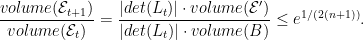
• One point to emphasize: the step of Ellipsoid cuts into two, and builds around the relavant half. Suppose , where is the unit ball. Then is some ellipsoid with volume at most times the volume of the unit ball. Now since any ellipsoid is a linear transformation of the ball, if , where is the associated linear transformation, then . But for any body , the volume of is . So

  

  In fact, you can imagine that each step we are just transforming the current elipsoid back to a ball, making a cut, and then transforming things back. One problem, of course, is that at each step we make the transformation more complicated. Indeed, in the notation above, if , then . So the numbers involved can get larger at each step: we may need to round the numbers to control how big they get. These and other numerical issues are at the heart of Khachiyan’s proof that the algorithm runs in polynomial time.

• My apologies: the alternate version of Ellipsoid I thought used boxes, in fact, uses simplices. The analysis that it runs in polynomial time is due to Boris Yamnitsky and (Leonid) Levin. The main idea is that half of some simplex can be contained in another simplex of volume at most times the volume of . (A proof appears in Vasek Chvatal’s book.) Note this factor is worse than the Ellipsoid factor of by another factor of , but the numerical calculations in the algorithm definition do not require the use of square roots. The original paper (also here) is not quite kosher, since it can lead to the size of the numbers blowing up: this report by Bartels gives an example, and also suggests rounding approaches to control the problem. Finally, some notes on the simplices algorithm by Yossi Azar (parts 1, 2) which I have not had a chance to go over in detail.

And a couple words about the center-of-gravity algorithm:

• The center-of-gravity definition. It’s the natural extension of the discrete case. Indeed, if we have objects in , the one having location and mass , the center of gravity (or the center of mass, or centroid) is defined as

  

  The continuous analog of this where we have a general measure over (basically replacing sums by integrals), is

  

  The numerator is the total measure over . (In class I was implcitly assuming the uniform measure over , which is given by .

  The in Grunbaum’s theorem (that each hyperplane through the centroid of a convex body contains at least fraction of the mass on either side) is best possible for convex bodies. And the proof is clever but not difficult See Grunbaum’s (very short) paper for examples and proof. Or these notes by Jon Kelner or Santosh Vempala.

  What happens if we don’t have the uniform measure over a convex body, but a more general distribution? Then things change quite a bit. E.g., consider equal point masses at the vertices of an -dimensional simplex. No matter which point you choose, you can find a hyperplane through it that contains only a single point (which is of the mass) on one side. Grunbaum actually shows (in the same paper) that you can find a point that ensures at least fraction of the mass on either side.

Lec #12: Notes on solving LPs

Notes for today’s lecture:

• Tightness of the Hedge guarantee. Consider the basic Hedge analysis, which says that for any , we have regret at most . Now if we were to set by balancing those terms, the regret bound would be . This is tight, upto the constant term.

  Let’s see why in the case . Suppose we again have two experts and , and are trying to predict a fair coin toss. I.e., every time the loss vector is either or with equal probability. So our expected gain is at least . But after coin tosses, with constant probability we have more flips of one type than of another, and indeed, the expected gain of one of the static experts is . So our regret cannot be less than even for two experts. Similarly for experts one can show that is necessary.

• Larger Range of Loss Vectors. For the setting where loss/gain functions could be in , we claimed an algorithm with average regret less than as long as . We left it as an exercise in HW3.

  In fact, you can prove something slightly weaker for the asymmetric setting where losses are in , where . In handwritten notes on the webpage, I show how to use a guarantee for Hedge to get

  

  as long as . The constants are worse, and there’s a term hitting the “best expert” term, but the analysis is mechanical.

  You can use this gurantee along with the shortest-path oracle to get an -iteration algorithm for -approximate maximum flow algorithm, since the gains will be in the range . More details below.

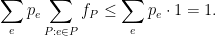
• The max-flow part was fast, here are some more details. We wrote the LP, and plugged it into the multiplicative weights framework. Since we had a constraint for each edge , the “average” constraint looked like:

  

  Flipping the summations, we get

  

  If we denote the optimal solution is to send flow along a shortest path, where the edge lengths are . We can find this using Dijkstra even though we cannot write the massive LP down. Since the “easy” constraints were , we send flow along this shortest path. Now we update the probabilities (edge lengths), find another shortest path, push flow, and repeat. At each step the gains will be in the range .

  So we can use the asymmetric losses analysis above. After -iterations, taking the “average” flow , we have that for each edge ,

  

  (How? chase through the LP-solving analysis we did in lecture, but use the above asymmetric analysis, instead of the standard symmetric one we used.)

  Finally, the flow is not feasible, since it may violate edge capacities. So scale down. I.e., define the flow : it has value and satisfies all the edge constraints. Viola.

• Next lecture we will do the improvement using electrical flows.

Lec #9:Notes

A few loose ends from yesterday’s lecture:

• The formula for computing inverses of a submatrix from the inverse of the whole thing is given by this:
  
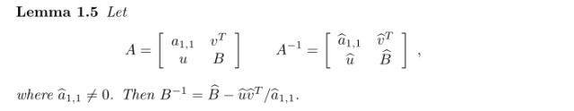
  (from this survey by Pawel Parys). A good explanation of the Mucha and Sankowski -time algorithm is in Marcin Mucha’s thesis.
• I looked at the Tutte paper again. The reason he was introducing the Tutte matrix (not his terminology) was to prove Tutte’s theorem (again, not his terminology). Namely, that a graph has a perfect matching if and only if, for every subset of vertices , the number of odd components in is at most . (Note that this is a special case of the Tutte-Berge formula.) Pretty cool that this 5-page paper introduced two important concepts.
• The proof of the isolation lemma went a little fast towards the end, so let me say it again. We wanted to bound the probability that an edge is confused, i.e., that the min-weight perfect matching containing has the same as that of the min-weight perfect matching not containing , by .So let’s give weights to all edges apart from . We can now read off the weight of the min-weight perfect matching not containing , say this is some constant . Moreover, if the weight of is eventually set to , then since the weights of all other elements is known, the min-weight perfect matching will have weight , where is another constant depending on the weights of other edges. So, for to be confused, we must have . And the chance this happens is at most , since we are choosing the weight for each edge independently from . Done.We will see how to use the isolation lemma in tomorrow’s lecture on smoothed analysis. (Slight change in lecture order, by the way.)
• By the way, the really useful part of the isolation lemma is that the weights are small, linear in the number of edges even though the number of matchings is exponential. E.g., if you assigned weight of edge to be , you would again get that the min-weight matching would be unique. But the weights would be exponentially large, which is undesirable in many contexts.

Lec #7: Notes

Today we saw several definitions and facts about polytopes, including proofs of the integrality of the perfect matching polytope for bipartite graphs. Some comments.

• We saw the definition of the perfect matching polytope for non-bipartite graphs (with exponentially many constraints), but did not prove it correct. Do give it a try yourself (or read over a proof via the basic-feasible solution approach which appears in my hand-written notes, or in these notes).
• We saw a definition of the -arborescence polytope (again with exponentially many constraints). As an exercise, show that is also an integral polytope via the vertex approach.

  Here’s how to go about it. In lecture #2, we saw an algorithm that finds the min-cost arborescence for non-negative edge costs. First, change it slightly to find min-cost arborescence for general edge costs . Naturally, gives you an (integer) solution to the LP . No reason to believe it is optimal for the LP, since this is the best integer solution and there may exist cheaper fractional solutions.

  Next, take the dual of this LP. If you show a set of values for the dual such that the dual value equals the primal value, then the integer solution you found is also an optimal solution to the LP. (How would you do it? Think of the prices we were defining at the end of Lecture 2.) Now the optimal solution being an integer solution is true for every set of edge costs. So the vertices of the polytope must be all integral.

  If this is a little vague, no worries: we will see the corresponding proofs for bipartite perfect matchings in the next lecture.

• Both the above LPs have exponential size. But has an “equivalent” poly-sized representation using some extra variables. Here’s a sketch. Indeed, the bad constraints are the ones saying that for every set not containing the root, . This is the same as saying that the min-cut between any vertex and the root is at least , when viewing as arc capacities. By maxflow-mincut, the maxflow from each vertex to the root (using arc-capacities ) is at least . So replace the exponentially many constraints by other constraints that enforce this max-flow condition. This may requires polynomially many extra variables. But “projected down” onto the variables the polytope is the same. This is another instance of the “projection example” I was attempting to draw in class. These things are called “extended formulations”.
• Does have a similarly small extended formulation? Recently Thomas Rothvoss showed that there are no tricks like the ones above, settling a decades-old conjecture of Yannakakis. In particular, every polytope that projects down to (for the complete graph ) must have constraints. See his slides/video for more details. As we remarked, this is an unconditional lower bound.
• For an extreme case when extended formulations help, Goemans shows a polytope with facets and extreme points that arises from projecting down a polytope in dimensions using facets.
• Finally, the use of total unimodularity for showing integrality of polytopes is indeed due to Alan Hoffman and Joe Kruskal. Here is their paper titled Integral Boundary Points of Convex Polyhedra, along with historical comments by the authors. Dabeen reminded me at the end of lecture that Edmonds and Giles actually developed a closely related concept, the theory of total dual integrality.

Lec #4: Notes

Some more notes about today’s lecture:

• We know that , and in a forthcoming homework we will remove this log factor. The reduction in the other direction is not that mysterious: given two matrices , , can you write down an vertex graph such that the in this graph gives you the MSP? Please post answers in the comments below.
• If you’ve not seen Strassen’s algorithm before, it is an algorithm for computing matrix multiplication in time . It’s quite simple to state, and one can think of it as a 2-dimensional version of Karatsuba’s algorithm for multiplying two numbers. Mike Paterson has a very beautiful geometric interpretation of the sub-problems Strassen comes up with, and how they relate to Karatsuba.

  The time for matrix multiplication was later improved by the Coppersmith-Winograd algorithm to get . Small improvements in the lower-order digits of were given by Andrew Strothers and (our own) Virginia Vassilevska-Williams.

  To answer Goran’s question, I looked over the original CW paper: it is presented as being similar to Strassen’s algorithm in that it breaks the matrices into smaller blocks and recurses on them. But the recursion is quite mysterious, at least to me. Recently, Cohn, Kleinberg, Szegedy, and Umans gave some group-theoretic approaches that use some of the CW ideas, but other seemingly orthogonal ideas, to match the CW-bound. They also give conjectures that would lead to .

• I was mistaken in claiming that for general directed graphs, the -approximate APSP is as hard as computing the exact APSP even for small values of . One advantage is that one can round all edge weights to powers of , and that gives a lot of room to play with. There are a lot of positive results in this setting, e.g., this paper of Uri Zwick, and a talk by him.